Cost Functions and Loss Functions in Machine Learning
Goal of Machine Learning
Machine Learning or Deep Learning can be viewed as function approximation based on data. What this means in simpler terms is that given a set of data points the aim is to get a function that can represent each of the data point very well and this function generalizes across many such similar data points.
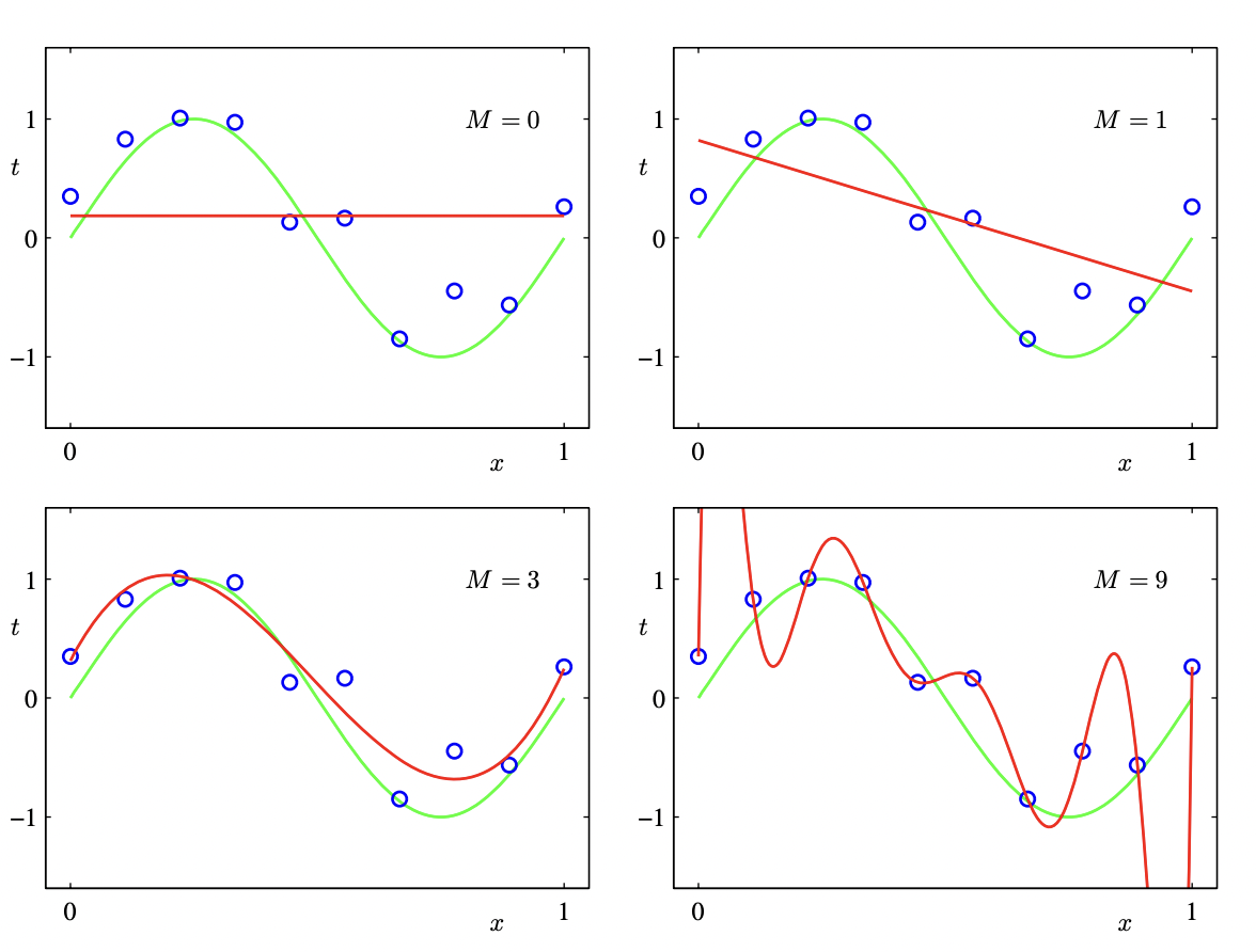
A simple polynomial curve fitting example is shown below. The idea of machine learning is to achieve something similar to left bottom figure so that there is a little bit of generalization or extrapolation that can be done if a sample comes from similar distribution.
 [1]
[1]
In case of the first diagram
Loss Function
Loss function is the function that can depict the error between the predicted function value at a data point and the actual value. Loss functions are measured over single datum points.
Cost Function
Cost function also denotes the error between predicted value and actual value but for a batch of data values.
Mathematical properties of Loss Function
For a loss function these mathematical properties are important
- Differentiable in real domain completely
- Possibly convex to ensure that there is a minimum, but in case of deep learning the loss function landscape will generally not be convex and we will have to do with the local minimum.
Common Loss Functions
- Cross Entropy Loss
Cross entropy loss is generally used for classification problems and can be expressed mathematically as
- Multi label classification
- Binary classification
where $y_i$ represents the label and $\hat{y}_i$ is the prediction for $m $ samples
- Hinge Loss
This loss function was developed for the SVM classification methods
\[L = max(0, 1 - y* f(x))\]- Mean Squared Error
Mean Squared error is generally used for regression based problems and can be represented mathematically as
\[L = \frac {\sum_{i=1}^{n} (y_i - \hat{y}_i)^2}{n}\]Basically computes the distance between the sample and prediction and then averages it over n samples
- Adversarial Loss function
Adversarial Loss is used in case Generative Adversarial networks where the discriminator and generator fight a zero sum game against each other.
\[\min_{G}\max_{D}\mathbb{E}_{x\sim p_{\text{data}}(x)}[\log{D(x)}] + \mathbb{E}_{z\sim p_{\text{z}}(z)}[1 - \log{D(G(z))}]\]where G is the Generator and D is the discriminator